We would like to reassure all our clients and partner organisations that PJA will be able to provide continuity of service throughout this period of home working and social distancing.

Due to the ongoing investment in our systems and as part of our existing commitment to flexible working, our IT infrastructure and project data is already held in a cloud environment and the majority of our staff already use mobile devices, which means that our teams can work from anywhere.

We have put in place additional measures to allow those staff normally reliant on fixed workstations to work remotely, and we also have the ability to host client’s own project data on our secure cloud servers if need be.

Our staff are already used to collaborating on projects virtually using Microsoft Teams, both within and outside the business, and our management systems are also cloud-based, so we are fully capable of delivering for our clients throughout this period of uncertainty.

If there are any specific measures we can put in place to assist our collaboration with your business during this time, please feel free to speak to the senior management team at PJA.

We wish all our colleagues well in the weeks and months to come.

PJA is backing the London Collective – a new collaborative approach to city making which enables built environment experts and creatives to work together. Set up by Max Farrell, former partner at international design firm Farrells, the Collective provides a platform for self-employed and SME built environment entrepreneurs to join forces, whilst also working on their own projects.

Since its establishment in November 2019, the organisation already has 28 members and is involved in several and commissions for UK and international clients. Max explained: “Our members have knowledge, experience and contacts covering politics, property and placemaking. As  entrepreneurs we can tailor-make teams without the overheads, enabling us to convene and disband teams for place-based campaigns, like a film’s cast and crew. “

PJA chairman and Collective member Phil Jones added: “The London Collective is a hugely powerful idea. Cities are enormously complex places but making them successful and sustainable is of vital importance. The range of skills on offer and the agility with which it can work means the Collective can play its part in achieving that goal.”


Following on from our posts on Dynamic Assignment and Convergence, we wanted to share our next modelling methodology. This focuses on standardised speed distributions used in microsimulation models.

As will be the caveat for all of these topics, these are not ‘set-in-stone’ methodologies and it may that there are other approaches out there. However, we wanted to share our approach to encourage improvement and provide guidance for those looking to start developing microsimulation models.

When developing a microsimulation model, one of the early steps is to ensure that the desired speed distributions used in the model are appropriate for the area and network modelled.

At PJA, we have a template which bases these initial distributions on two key datasets – the Department for Transport’s (DfT) ‘vehicle speed compliance’ tables and Transport for London’s (TfL) speed profiles.

DfT Speed Statistics

Using the DfT SPE011 2018 dataset (last updated 26th June 2019) , the following speed profiles have been calculated:

  • 20mph Built Up Roads;
  • 30mph Built Up Roads;
  • National Speed Limit (60mph) – Single Carriageway Road;
  • Motorways (70mph).

The data has been obtained from the following link:

https://www.gov.uk/government/statistical-data-sets/vehicle-speed-compliance-statistics-data-tables-spe

40mph Speed Limit

Due to no data being available for a 40mph speed limit from the SPE011 dataset, a previous DfT dataset has been utilised – DfT SPE0102 2014 dataset (latest available data).

This data has been obtained from another engineering consultancy, in collaboration on a microsimulation project.

Dual Carriageways

Due to no data being available for a 70mph dual carriageway, an archived DfT dataset has been utilised – DfT SPE0111 2009 dataset – Table TRA9906 (latest available data):

The data has been obtained from the following link:

http://webarchive.nationalarchives.gov.uk/20110218142807/http:/dft.gov.uk/pgr/statistics/datatablespublications/tsgb/

TfL Speed Profiles

As the DfT datasets provide no information on 10mph or 50mph speed limits, these profiles have been based on the latest TfL VISSIM template that we are in possession of (VISSIM Template v5).

An example of the speed profiles calculated is shown below:


Figure 1 – 30mph Speed Profile Examples

Don’t forget about Localised Speed Profiles

Whilst the DfT and TfL speed profiles provide a good starting point for developing a base microsimulation model, consideration should be given to the use of more localised speed distributions based on ATC data.

We previously had a project where the 40mph speed limit was affecting the journey time validation of the model. All reduced speed areas and priority rules were deemed appropriate, meaning the speed profiles were considered a case for review. We created a new speed profile using the following methodology:

  • Identify an ATC in a location that would experience ‘free flow’ speeds for the speed limit required
  • Extract the hours of 0000 – 0600hrs* for either the day or the survey or the neutral days (Tuesday / Wednesday / Thursday) of the week surveyed
  • Identify the Minimum and Maximum times from the range of data for your speed profile
  • As a minimum, calculate the 85th percentile (%ile), 50%ile, 25%ile and 75%ile to create the speed profile for VISSIM input

*The 0000 – 0600hr time period was used to allow a ‘free flow’ speed profile to be determined, away from more congested peak periods.

The end result was a better representation of the local speeds and a much-improved journey time validation that met TAG criteria.

Final Comments

The use of DfT speed statistics and TfL speed profiles are useful starting points in developing a base model for calibration and validation.

However, the use of more local speed profiles can play their part in providing more site-specific operation and a more representative performance of local conditions.

Finally, remember to check back to the DfT website to ensure that you are using the most up-to-date profiles, as these tend to be updated on a yearly basis.

Introduction

Following PJA’s attendance at the PTV User Group in London on 4th November 2019, one of the key messages that we took away from the conference was the importance of model convergence and understanding the levels of convergence achieved before running for results.

At PJA, we use PTV VISSIM on a daily basis and are all too familiar with model convergence, the difficulties faced as models get bigger and more complex. As a result, we have produced this post to go into detail on what the current convergence guidance is, what methodology we adopt, the limitations with it and a proposed revised approach to demonstrate model convergence.

VISSIM Model Convergence

Current Guidance

As a recap, convergence criteria for VISSIM models is best summarised in TfL’s MAP Engineer Guide v3.5 (http://content.tfl.gov.uk/map-v3-5-engineer-guide.pdf), P140 as shown in Figure 1.
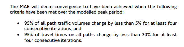
Figure 1 – TfL Convergence Criteria

Current Approach

Whilst VISSIM has a built-in ‘pop-up message’ for to highlight when convergence has been achieved, we rarely see this! This is likely due to our convergence method focusing on more than one parameter, which is required following TfL’s guidance – see set-up in Figure 2).
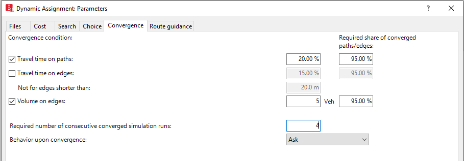
Figure 2 – Covergence Set-Up in Dynamic Assignment

Our microsimulation models also contain elements such as vehicle actuated signals and pedestrian demand inputs. These can cause slight variances in signal timings from seed run to see run, which in turn affects the level of convergence.

As a result of the above, our current approach to assess convergence is to use two outputs:

  • The *CVA file generated by VISSIM to check the volume and travel time differences
  • The ‘Total Travel Time’ value from the Network Performance evaluation to check the overall network difference.

The volume and travel time differences from the *CVA file are compared against the criteria in Figure 1. The 1% difference check for Total Travel Time is based on previous DMRB guidance which required the “change in user costs or time spent within the network should be less than 1% for four consecutive iterations”. We acknowledge that this has now been withdrawn but it is still a useful measure to demonstrate model stability, and has never been queried at audit.

Figure 2 shows an example of the summary convergence table we produce and Figure 3 shows an example of how the path/edge volume and travel time percentages are created (using Seed Run 20 from Figure 2).

Figure 3 – PJA Convergence Method

Figure 4 – Example Calculation of Convergence Levels – Seed Run 20

The main reason for using this method is that it allows the volume and travel time differences to be checked for both paths and edges, which in turn can be compared against the TfL criteria.

The built-in VISSIM convergence checks allows the travel time on paths to be compared but doesn’t have the option of checking the volumes on paths (only a comparison on edges).

Convergence Method Limitations

Whilst our convergence methodology allows the travel time and volume differences for paths and edges to be determined, there are caveats associated with this.

From Figure 3, the immediate query with the calculations is why the percentages generated by VISSIM at the bottom of the file (ShConvPathTT and ShrConvEdgeVol) are not the same as those that we have manually calculated.

In reference to the PTV VISSIM FAQs link (http://vision-traffic.ptvgroup.com/en-uk/training-support/support/ptv-vissim/faqs/, Dynamic Assignment – #VIS29422), the differences are explained as follows:

“Note: A path is converged if the convergence criterion is met in all time intervals. From the *.cva file, you cannot recognize if the paths that converged in one time interval are the same that converged in another.”

This implies that the *CVA file only shows the numbers of paths/edges that fall within the travel time/volume differences, but these edges/paths could be different between the different time intervals.

As a result, the VISSIM-defined percentage at the bottom of the *CVA file should be considered a more accurate measure of the model convergence as this accounts for edges/paths that converge between successive time intervals.

The remaining barrier to overcome is how to deal with the comparison of the path volumes, which is not automatically calculated within the *CVA file.

Revised Methodology

Introduction

In light of the limitations highlighted above, we have spent some time researching into other ways to check the level of convergence of our models. The result of this is a revised methodology that uses both the built-in tools from VISSIM and some additional manual calculations.

Research Undertaken

Our first port of call was to review the PTV VISSIM help document and the online FAQS link to understand.

The VISSIM FAQ link (Dynamic Assignment – #VIS29422) provides the following advice:

“…you can open the Paths list in PTV Vissim (Traffic > Dynamic Assignment > Paths), and if you add the attribute Converged (Conv) to this list, then you can see if the path is converged or not.”

We looked into what the ‘Converged’ attribute entailed within the Paths list and from the VISSIM User Manual, the following definition is given:

“If this option is selected, the travel time of the path is converged. The path fulfils the convergence criterion Travel time on paths for all completed time intervals.”

It is important at this stage to note that this ‘converged’ attribute only considers the travel time on paths and does not account for the volume on paths.

However, the Paths list within VISSIM does allow you to select a range of other attributes – most importantly the Volume (new) and Volume (old) attributes for each evaluation interval, which is the additional convergence check recommended by TfL.
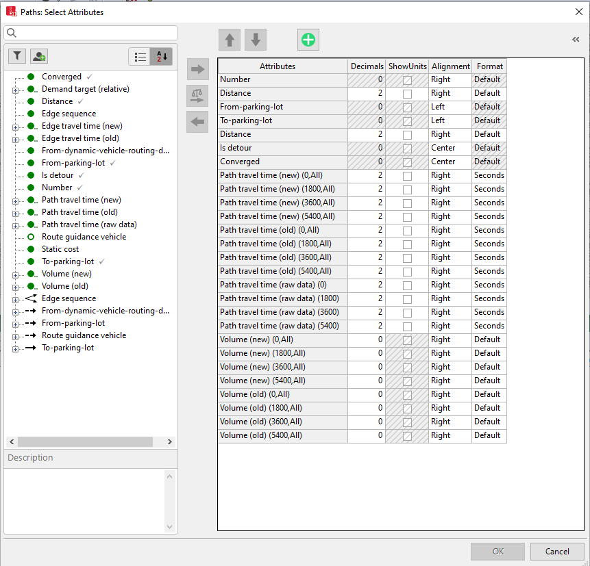
Figure 5 – Paths List – Attribute Selection

From Figure 5, it should be noted that, in order to correctly calculate the same ShConvPathTT value as in the *CVA file, you need to compare the ‘Path travel time (old)’ and ‘Path travel time (raw data)’ across all evaluation intervals.

Revised Approach

As a result of a review of information available, we have revised our approach to checking convergence of Path Travel Times and Volumes.

In the first instance, instead of using the *CVA file, we now utilise the Paths list. This is output for each convergence run (using the ‘autosave after simulation’ function) with the list layout as shown in Figure 5. It should be noted that the Network Performance outputs will continue to be collected to check the Total Travel Time differences between each seed run.

Path Travel Times

For the Travel Times, five different checks are undertaken and two of these are used for reporting purposes.

Check 1 – this simply uses the built-in ‘Converged’ check within VISSIM and calculates the percentage of all the paths that meet this criterion. This is NOT used for reporting as the calculation includes detours, which are not strictly a path within the model.
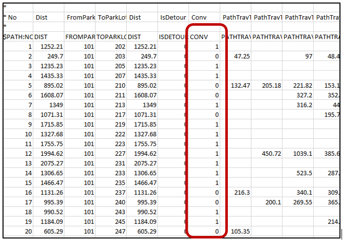
Figure 6 – Path Travel Times – Check 1

Check 2 – this expands on Check 1 and considers if the path is a detour or not. If a path is converged and NOT a detour, then it is considered as part of the analysis. The outcome of this check is a more refined percentage of paths which converge and IS used for reporting.
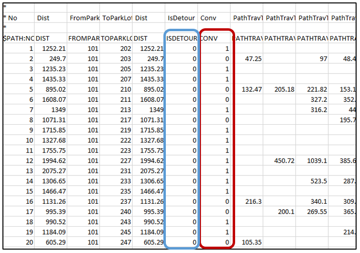
Figure 7 – Path Travel Times – Check 2

Check 3 – for each of the various evaluation intervals (defined in the Dynamic Assignment tab), a check is made of each path (which is NOT a detour) to identify if the difference in travel times is within 20% when considering the ‘Travel Time Old’ and the ‘Travel Time Raw’. This check returns a simple ‘YES’ or ‘NO’ for each evaluation interval and for each Path.
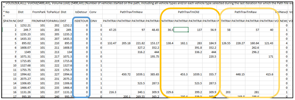
Figure 8 – Path Travel Times – Check 3

Check 4 – this expands on Check 3 and assesses if a Path has a travel time difference within 20% for each evaluation interval. If this is ‘YES’ for all the evaluation intervals, then the overall outcome is ‘YES’. If one of the travel times is greater than 20%, then the outcome is ‘NO’.  An indicative percentage is also provided on the numbers of paths that converge in all evaluation intervals.

Check 5 – this further expands on Checks 3 and 4 and looks at the ‘NEW’ path volumes for each evaluation interval, with a ‘NEW’ total flow calculated for each path. The outcomes of Check 4 are then used, with each path that converges across all evaluation intervals added together to give a total number of converged paths. This is then divided by the total flow to give the ‘Share of Converged Path Travel Times’. This IS used for reporting.
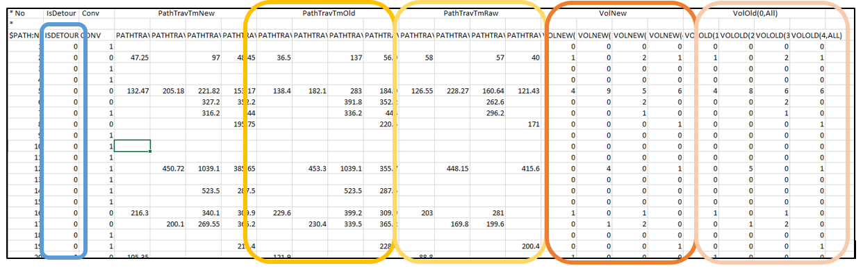
Figure 9 – Path Travel Times – Check 4 & 5

An example format of Checks 1-5 is shown in Figure 10.
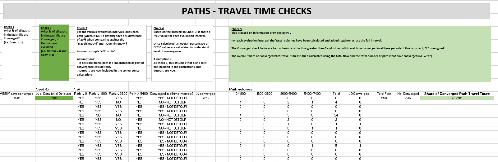
Figure 10 – Path Travel Times – Example of Check 1-5 Calculations

Path Volume Checks

For the Volume checks, two different checks are undertaken and one of these is used for reporting purposes.

Check 1 – this looks at paths which are not detours and for each evaluation interval, calculates if the difference between ‘Volume NEW’ and ‘Volume OLD’ is within 5% . This returns a ‘YES’ or ‘NO’ for each evaluation interval and each path. This is NOT used for reporting.
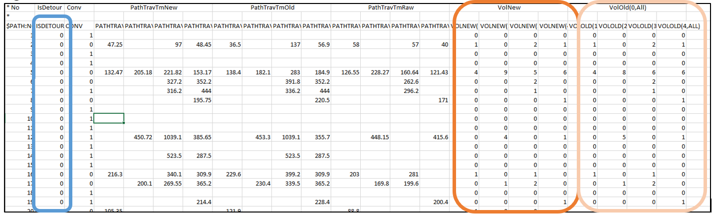
Figure 11 – Path Volumes – Check 1

Check 2 – this expands on Check 1 and checks if there is a ‘YES’ for each evaluation interval for each path. This gives a result of either ‘YES’ or ‘NO’. A summary percentage of paths which have a flow difference of less than 5% for each evaluation interval can then be calculated. This IS used for reporting.

An example format of Checks 1 and 2 is shown in Figure 12.
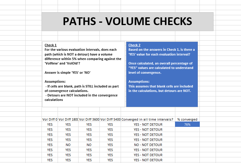
Figure 12 – Path Volumes – Example of Checks 1 & 2 Calculations

An example of the revised summary table can be seen in Figure 13.
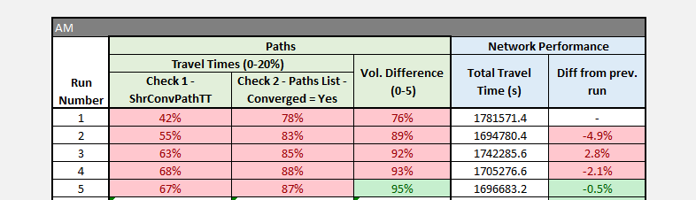
Figure 13 – Updated Convergence Summary Table

This summary table now takes into account two checks of the Path Travel Times, using both manual calculations of the ‘ShrConvPAthTT’ percentages and also a check of the built-in ‘Convergence’ check in the Paths list. It also calculates the Path Volume Difference percentages, using manual calculations of the ‘NEW’ and ‘OLD’ volumes. Finally, there remains a check of the Total Travel Time within the network. This is taken from the Network Performance outputs and a 1% difference is checked. This is retained as a legacy DMRB convergence criterion and is seen as a good way of further demonstrating model stability.

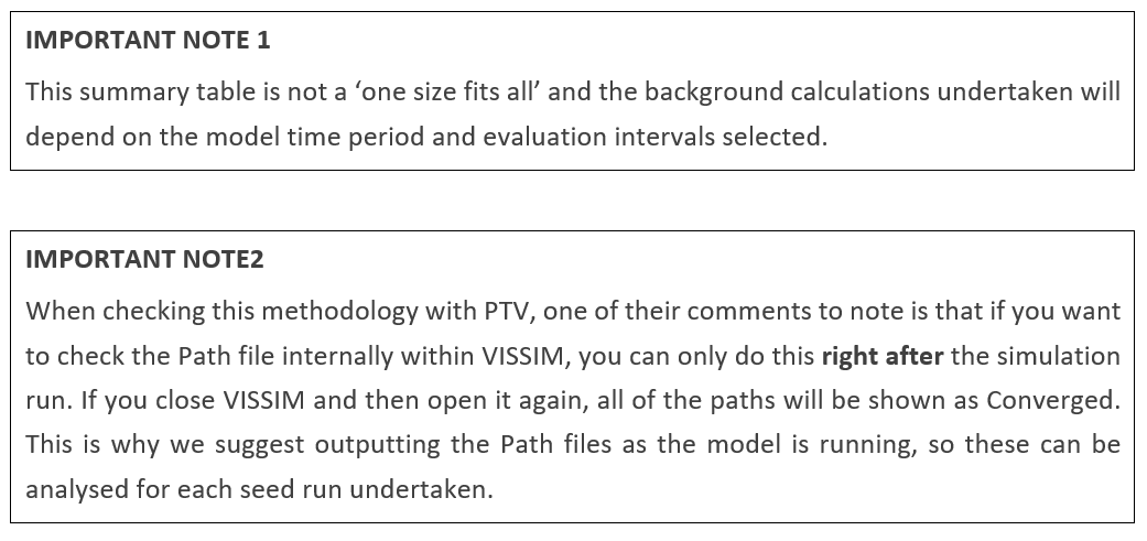
There are two important notes to consider.

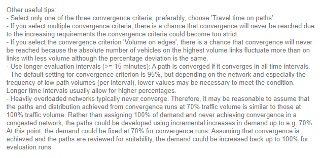
Other Convergence Considerations

Depending on how complex your model is, there is a chance that your model will not achieve the required percentages to be considered ‘converged’.

The VISSIM FAQ link (Dynamic Assignment – #VIS29421) provides the following advice:

From the points above, the are two in particular which we would recommend trying to help with model convergence.

  • Using longer evaluation intervals – we typically ensure these are at least 900s (15 minutes). This allows vehicles to complete their journeys, so that the complete journey time can be considered in further evaluation intervals. In the PTV Manual, values of 900-3600s (15-60 minutes) are recommended to account for delays and variance in journey times. Where signals are modelled, the evaluation interval should also be significantly longer than the cycle times used.
  • Reducing the traffic volume in congested networks – whilst we think that reducing to 70% of the demand may be a bit too extreme, we would suggest values of 80-85% would be more suitable. This is still likely to give a suitable distribution of traffic around the network, whilst also improving the percentages met of the convergence criteria. It should be noted that we have not explicitly used this method in any project work to date, but is something we will look to use in future (subject to approval from any external auditors of the model).

Outside of the PTV Manual, we can also offer the following suggestions for models that do not fully converge.

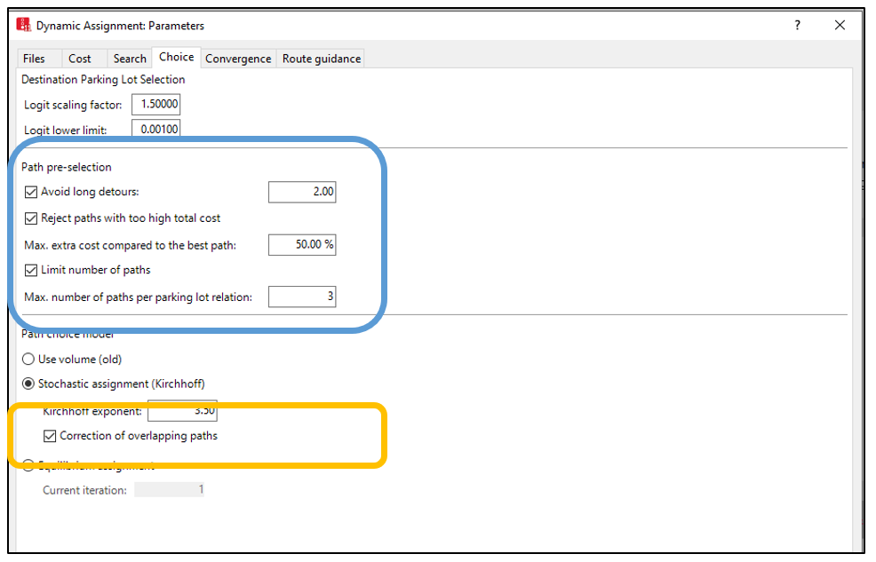
  • It’s worth spending time up front to set up your Path pre-selection criteria correctly. Depending on the size of the network, you need to consider how many realistic alternative routes there are and how likely it is that drivers will deviate away from the main route. It may take a few iterations when initially creating your path file to get this right, but this should help further down the line. Also, always ensure that ‘Correction of overlapping paths’ is ticked to avoid any unrealistic routes from being included.
  • If after a significant number of runs (say 100) and a review of the convergence percentages show that the model has still not converged, there are still options available. You can continue to run the model for more runs to see if this improves the convergence levels. Alternatively, if the review of the convergence percentages shows little variance from run-to run, this suggests that the model has reached a ‘best as it’s going to be’ In this case, depending on how close the percentages are to the target criterion, another approach is to run a greater number of results runs to counteract the reduced convergence. The reasoning behind this is that the more results there are to take an average from, the lesser the effect of any significant variance in the seed runs. As TfL now require 20 seed runs as a minimum for reporting, we would look to run for 30-40 seed runs (or more), depending on the convergence levels achieved.

Summary & Conclusions

We hope this post has provided some insight into general VISSIM model convergence, as well as providing details on our current methodology and how we can improve upon this further with better manipulation of the Paths list.

As VISSIM models become more complex and more detailed (for example, including Vehicle Actuated (VA) signals, pedestrian inputs, multiple route choice), we hope that this post has provided some thoughts and suggestions on different techniques to improve the convergence levels.

As always, we welcome any comments and feedback from other users so that we can continuously improve how we converge models and analysis the outputs to demonstrate a suitably stable model.


Dynamic Assignment in VISSIM

The use of dynamic assignment in VISSIM models can be considered a ‘dark art’, with very little content online which demonstrates how to go about this process and what the key elements are to look out for.

As a result, we wanted to share our thoughts and current methodology to a wider audience. We are aware that there is no ‘one best solution’ to undertaking dynamic assignment, but hope this helps to generate further debate and/ or improvement and provide some help to those who are looking for a starting point with dynamic assignment.

A bit of background…

Before the introduction of Equilibrium Assignment in VISSIM 9, VISSIM models developed with dynamic assignment routing were generally configured to use the Kirchhoff (Stochastic assignment) option, with user specified ‘path pre-selection’ parameters and an MSA (Method of Successive Averages) option for Cost Running (see Figure 1).

However, in VISSIM 9, we now have the introduction of Equilibrium Assignment, which in our experience has muddied the waters a little bit. We understand the premise of it (balancing the traffic flows between paths to favour the less congested routes) but having tried to use it on a previous project, we could not develop a suitable path file for meeting TAG calibration and validation criteria.

This may have been down to us not fully grasping the concept and choosing appropriate supporting path search criteria, but in the end, we chose to use the Stochastic Assignment in order to continue getting the results we wanted.

Step forward to now…

We have been working on a model of a small town, with route choice required to be modelled to asses the impact of proposed relief road options in a future year. We followed our normal Stochastic Assignment routing methodology and together with link/ connector surcharges, produced a calibrated and validated model. However, when it came to assessing the impact of the future year relief roads, the added surcharges were causing problems, with the new path files not producing routes as expected.

We were then faced with two options – 1) remove the surcharges and proceed with Stochastic Assignment (which then becomes a grey area as the model is calibrated and validated with these surcharges in place), or 2) explore the use of Equilibrium Assignment to see if this produced more sensible paths (which also meant removing the surcharges and if successful, re-checking the base model calibration/ validation levels with this assignment option in place).

We decided to proceed with option 2) on the basis that, if we could get a calibrated and validated base model without needing surcharges, then it would make the future year testing a more straight-forward process.


Stage 1 – Equilibrium Assignment – Path File Running

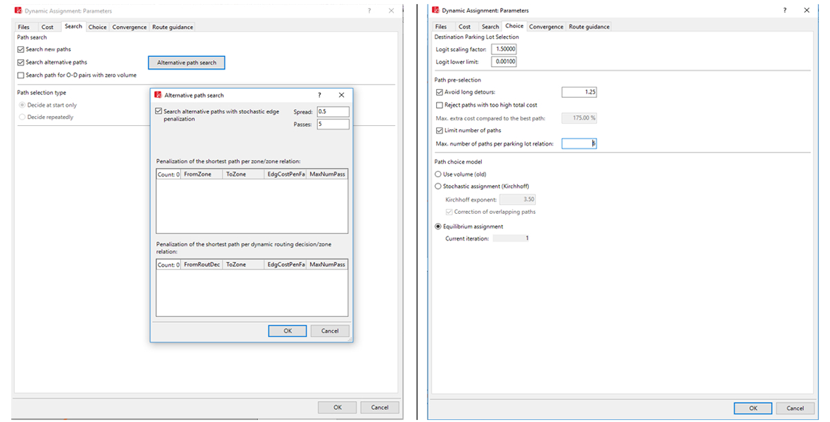
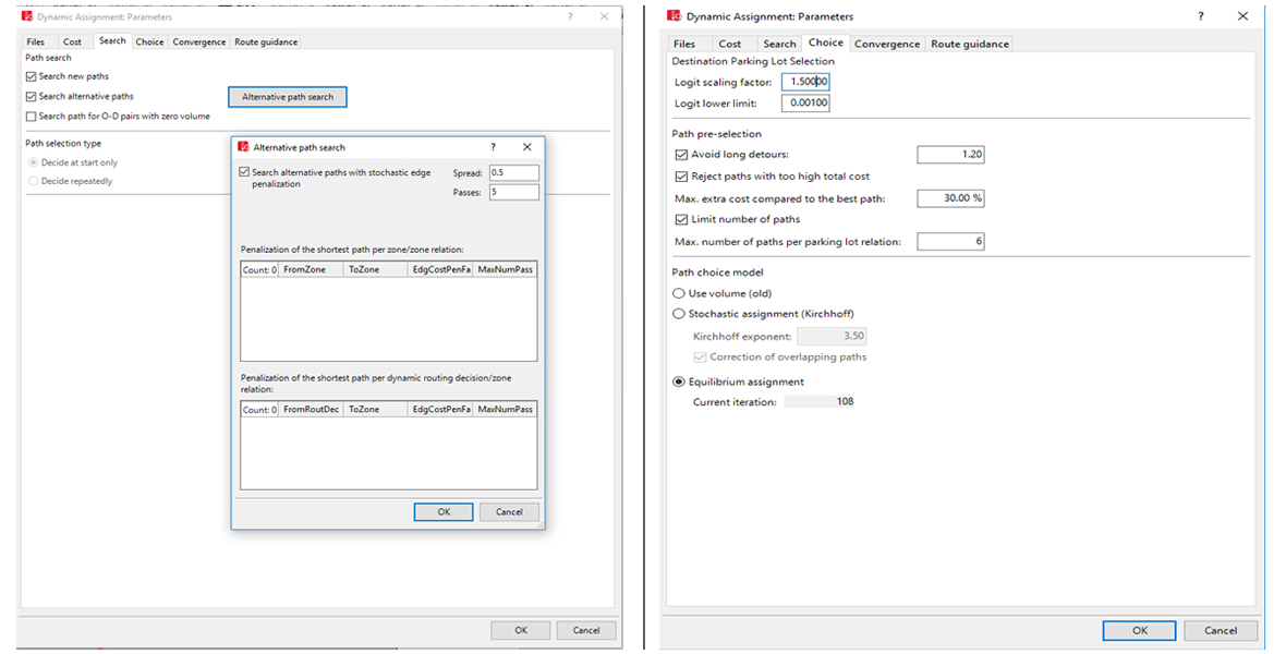
We set up the model to run for an initial path file, with the configuration set out in Figure 2.

Figure 2 – Equilibrium Assignment Parameters – Path File Running – VISSIM 9

The key points to note on the path file running:

  • We are not storing for Costs and not penalising routes with excessive cost – this produced a better initial path to take forward for Cost running.
  • We had to undertake a couple of iterations to ensure that the ‘Avoid Long Detours’ factor was suitable for our network. A factor too high produced unrealistic paths, whilst a figure too low didn’t find enough suitable paths.
  • The models were run using a reduced demand to start with and then increased through multiple runs of different seeds.


Stage 2 – Equilibrium Assignment – Cost File Running

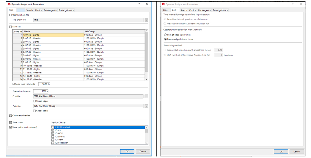
We set up the model to run for an initial cost file, with the configuration set out in Figure 3.


Figure 3 – Equilibrium Assignment Parameters – Cost File Running – VISSIM 9


The key points to note on the cost file running:

  • Store Costs’ and ‘Reject paths with too high cost…’ options are now selected as we now wanted the cost and path file to take into account the costs on routes.
  • We continued to run the cost file with ‘Search New Paths’ As we ran creating archive files, we found that even with this ticked, the size of the path file eventually stabilised through multiple seed runs.

As with the path file, the models were run using a reduced demand to start with and then increased through multiple runs of different seeds. This was done over a large number of seed runs to ‘bed in’ the cost file and allow variance between the runs to be accounted for over a larger sample size. We also chose to collect the ‘archive files’ and direct ‘convergence’ outputs from the model, so that we could track the file size of the *BEW file and interrogate the *CVA files to understand how stable the cost file was.


Stage 3 – Equilibrium Assignment – Convergence Running

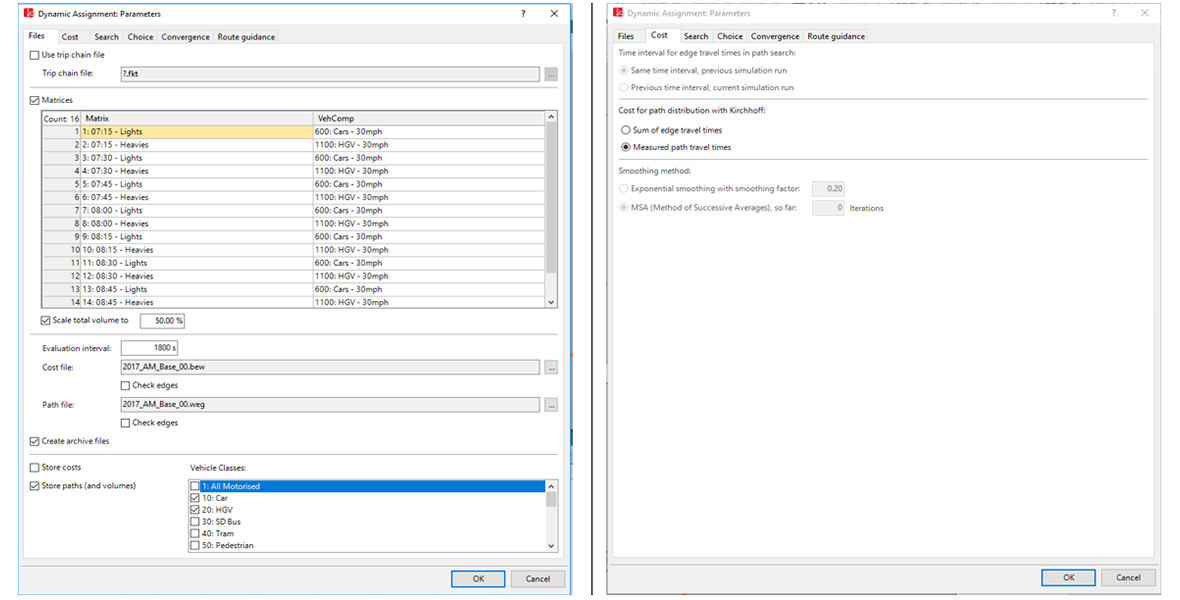
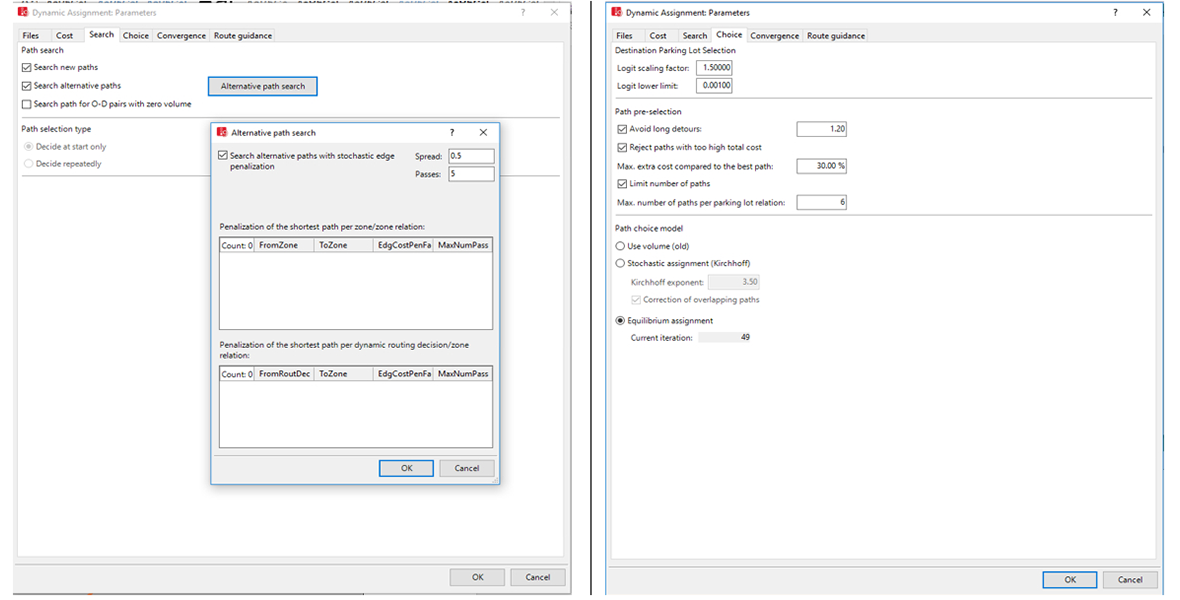
We set up the model to run for convergence, with the configuration set out in Figure 4.

Figure 4 – Equilibrium Assignment Parameters – Convergence Running – VISSIM 9


The key points to note on the convergence running:

  • The ‘scale total volume…’ is unticked so that 100% of the traffic is run each time.
  • We continued to have the ‘Search new paths’ option ticked. As our model contained decimal numbers in the O-D matrices, having this ticked removed previous errors of missing vehicles when running for multiple seeds. We also found that, as with the cost file run, by reviewing the archived files, the path file was not changing from run to run and not having a significant effect on the convergence of the model. It should be noted that, if the matrices are made up of whole numbers (i.e. no decimal places), then ‘Search new paths’ should be unticked.
  • The model was run multiple times whilst exporting both the network performance and direct CVA outputs, on the same seed to check convergence against TAG


Stage 4 – Equilibrium Assignment – Results Running

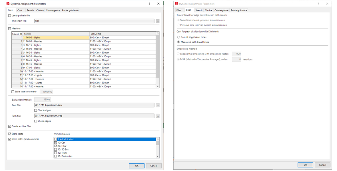
We set up the model to run for results, with the configuration set out in Figure 5.


Figure 5 – Equilibrium Assignment Parameters – Results Running – VISSIM 9


The key points to note on the results running:

  • The option to ‘Store Costs’ is now unticked as we want to preserve the cost file chosen as most suitable and stable from the Convergence running analysis.
  • We continued to have ‘Search new paths’ options ticked due to the O-D matrices having decimal places. This removes the errors of vehicles not being able to leave the parking lot, without affecting the path file. It should be noted that in ‘normal’ circumstances, the O-D matrices will be made up of whole numbers (i.e. no decimal places), meaning ‘Search new paths’ does not need to be ticked. This preserves the path file chosen from the Convergence running analysis.
  • The model was run multiple times on different seeds to obtain a suitable average for results reporting.

The Outcomes…

Convergence

Following the process detailed above, the convergence results obtained are shown in Figure 6.

Figure 6 – Equilibrium Assignment Parameters – Convergence Results – VISSIM 9


It can be seen that majority of the TAG convergence criteria was met, with the Volume Difference and Travel Time on Edges problematic (in our experience, notoriously so on many models) in the AM peak.

Calibration & Validation

In terms of the calibration and validation results, the flow and journey time results were improved over the Stochastic Assignment method.

Future Year Testing

Taking this Equilibrium Assignment methodology forward into the future year testing, the traffic assignment as a result of proposed relief roads appeared much more realistic and produced results which were more in line with what was to be expected. The lack of surcharges to inform route choice certainly seemed to help traffic reassign more freely around the network.

Final Thoughts…

The use of Equilibrium Assignment for Dynamic Assignment routing certainly seems to have its advantages, particularly in models with route choice. That being said, there has been some lessons learned in terms of how important it is to get the path pre-selection parameters correct to start with and the need to have ‘store costs’ and ‘search new paths’ checked throughout the whole process.

As mentioned at the start, this is certainly not the only approach to undertaking dynamic assignment and may still require further refinements. However, with recent queries on the subject, we felt it was worthwhile producing something to demonstrate how Equilibrium Assignment has been successful and what methodology and parameters were used/checked to achieve our goal.

We hope this helps and please feedback with any comments.

Extended Thoughts…What about Stochastic Assignment?

Whilst this post has specifically focused on Equilibrium Assignment, what about if you want to use Stochastic Assignment as your choice of path model?

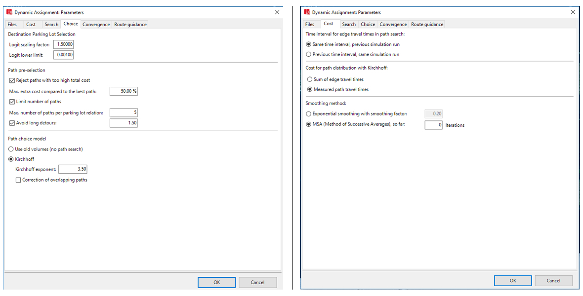
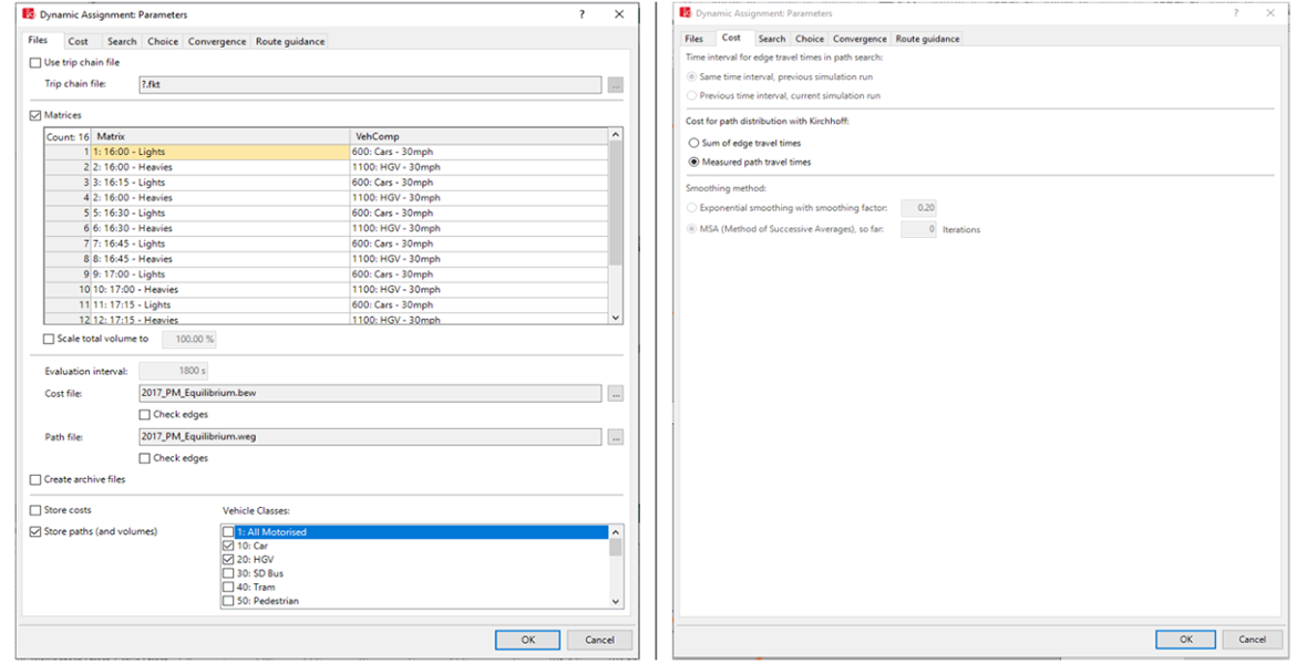
Well, the steps already identified can still be followed and the key differences in the dynamic assignment set-up are shown in Figure 7.

Figure 7 – Stochastic Assignment Parameters

The key differences to note are:

  • Within the ‘Choice’ tab, the Stochastic assignment (Kirchhoff) has been chosen instead of Equilibrium Assignment
  • Within the ‘Cost’ tab, the following change are made:
  • The cost for path distribution is amended to ‘Measured path travel times’
  • The smoothing method is set to ‘Exponential smoothing’ with a default value of 0.20.

The use of ‘Measured path travel times’ over ‘Sum of edge travel times’ is based on guidance in the VISSIM manual. This states that for links with multiple lanes and for congested networks, the measured path travel times produces more accurate results.

For the smoothing method, the ‘Method of Successive Averages (MSA)’ can be chosen. If using this method, it is important to update the number of iterations after each stage of the dynamic assignment process. For example, if the model is run 20 times for paths, 20 times for costs and then 100 times for convergence, the following MSA values should be entered – 20, 40 and 140 iterations.


Hope this helps and any questions or comments, do get in touch!